

This Matrix introduction covers a brief review of the mathematic notation used for Matrices and what makes them useful as vectors and data structures. Once you have a basic understanding of matrices, you can learn about its properties and use in computer programs. Moreover, you will learn the different types of matrices and how to change them.
Mathematical notation
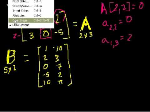
In the world of mathematics, a matrix is a two-dimensional array of numbers. It is composed of rows and columns. In addition, it is also known as a vector. Matrix algebras are important mathematical systems. They are composed of a variety of different variables.
In the early twentieth century, matrix notation and vector notation were widely used in textbooks. Florian Cajori’s 1929 History of Mathematical Notations based on Thomas Muir’s 4-volume The Theory of Determinants in the Historical Order of Development used matrix notation. Later, he produced a supplement in 1930 that brought the story up to the twentieth century.
The term matrix was coined by James Sylvester in the 1840s. Other scientists and mathematicians developed this theory, including Arthur Cayley. The first applications of matrices were to solve linear equations. The field of matrices has continued to grow ever since.
In addition to being the inverse of differentiation, the matrix can perform the discrete equivalent of integration. In fact, it is the most versatile and flexible of all the operations available in linear algebra. For example, in solving the “Matrix Chain Problem”, the goal is to minimize the number of scalar multiplications and columns.
A matrix is a rectangular array made up of numbers. Each number is called a matrix entry. The rows and columns of a matrix are arranged according to a specific symmetry. This symmetry allows the matrix to represent linear transformations and functions. For example, it can calculate the determinant of a vector.
Matrices as data structures
Matrices are data structures composed of two-dimensional arrays of numbers. Each element of the array is identified by an index. These matrices can be sorted, queried, concatenated, and deleted. They are most often used in operations that govern linear algebra. For example, if there are three columns and three rows, the array contains three values.
Matrices are a special kind of array. They have two dimensions and can have different types of columns and rows. You can use functions to manipulate matrices such as rownames() and colnames(). You can also perform operations on them, such as addition or multiplication using the %*% operator.
Another type of matrix is a sparse matrix. This type of matrix contains more ZERO values than non-zero ones. These matrices are typically stored as sparse ones. This makes it easier to access the individual elements and is better for memory performance. However, it becomes more complex to recover the original matrix, requiring additional structures.
Matrices as data structures are widely used in computer programming and in many internet applications. They are also used in public key cryptosystems. The speed of decryption is a key concern with public key cryptosystems. Almost any quantitative field of work will make extensive use of matrices. Matrices are also commonly used to solve linear equations. These equations consist of unknowns to a first power multiplied by a constant.
Matrices as determinants
A determinant is a scalar value that is a function of the entries of a square matrix. This property allows us to analyze the properties of the matrix and the linear map it represents. Determinants are useful in many mathematical applications. For example, they can be used to calculate the slope or the mean value of a curve.
Determinants are useful in solving linear systems of equations. They are calculated using a square matrix whose columns are the vectors. These matrices are orthogonal, and the determinant determines whether they are orthogonal to the standard basis of Euclidean space.
Jacobi was one of the first to use the word “determinant” in this modern sense. He wrote three papers on determinants that made the concept widely known. However, it took much longer before this idea could become widely accepted. A modern definition of a determinant was not published until the 1950s.
A determinant is the characteristic polynomial of a matrix. It is also called an eigenvalue. It is used in calculus and is an important tool in the solution of linear equations. However, other methods of solving problems are more efficient. One method of using a determinant is Cramer’s rule. This involves dividing two matrices and finding the x and y-coordinate pair.
The determinant of a matrix is zero if any column in the matrix can be expressed as a linear combination of other columns. Likewise, a determinant with a zero value is a determinant that changes by one digit. This property makes determinants multilinear.
Matrices as vectors
Vectors are arrays of numbers, and they are often used to represent data. The mathematicians use them to simplify the solution of three-dimensional problems. Vectors are also used in physics to express various quantities. They have two properties: magnitude and direction. These properties are equivalent. They are also used in physics to represent many quantities, such as speed.
The fundamental difference between matrices and vectors is their mutability. The former are not editable once created, but operations on them create a new instance. This makes looping over them with direct access very inefficient. Working with these raw structures is not trivial, but you can use specialized enumerators to understand their layout. Most functions also offer a method to skip zero-value entries, which speeds up execution in sparse layouts.
The same method can be used to compute the inverse of a matrix. First, take the matrix and divide its components into its columns. This produces a matrix with two columns. Then, take the inverse of the matrix. Afterwards, multiply the inverse matrix by the inverse, and you’ll get a matrix of two columns and one row.
Matrix-vector multiplication is easy to apply. In matrix multiplication, the columns of a matrix are equal to the number of columns. Thus, the product of a three-dimensional matrix by a three-dimensional vector will be a three-dimensional vector.
Eigenvalues
Eigenvalues in a matrix are non-zero vectors that change when a linear transformation is applied to a matrix. These vectors are often denoted with the letter lambda. The corresponding eigenvalue is also called the eigenvector and is usually scaled by a certain factor.
Eigenvalues in a matrix are often used to compare two or more matrices. However, this is difficult because matrices are huge and their values are complex. Eigenvalues are a part of prime factorization, which is the process of turning a matrix into a product of other matrices with well-defined properties. When comparing two or more matrices, it is helpful to use eigenvalues to determine the smallest eigenvalue.
Eigenvalues can be computed using Wolfram Language. You must know the matrix’s dimensions and the number of eigenvalues. You can compute these values by using the Eigensystem command in Wolfram Language. Then, you can multiply the eigenvalues by the matrix.
Eigenvalues in a matrix are scalars associated with a linear transformation in vector space. The eigenvalue is equal to the vector derived from this transformation. An example is a matrix containing the eigenvalue l. In this case, l is the eigenvalue of matrix A. The identity matrix i has the same order as A.
The eigenvalues of a matrix are the nonzero vectors that lie on the same line through the origin. An eigenvalue can be calculated in a variety of ways, including by drawing a picture of a matrices and examining which ones haven’t been displaced from their original line.
Transpose matrices
In linear algebra, the transpose operator flips the diagonal of a matrix. This operation is one of the most important when working with matrices. However, there are many other operations that can be done with matrices as well. The following are some of the more commonly used ones.
The transpose operator can be used in many different ways, including reversing the rows or columns of a matrix. This type of transformation is especially useful when working with adjoint or inverse matrices. When using this type of operation, the user must know what the transposed matrix is.
In transposing a matrix, the number of columns in the original matrix must be less than the number of rows. To do this, the original matrix must have a column at row r column c. This means that an element called arc in the original matrix becomes acr in the transposed matrix.
The transpose matrix of a matrix A is a form of A that has degree 4i. A transposed matrix p(O) has a p-value of zero, which means that it is independent of the local frame. The transpose matrix dpi is then the same as the original matrix.
Transposing a matrix is a straightforward operation. To transpose a matrix, the diagonals of the original matrix are replaced by rows. The auxiliary space of the new matrix is increased. The time complexity of the transposition operation is O(M x N).


